How to Choose the Right Estimator

Table of Contents

Criteria for Model Selection #

Selecting the right model in machine learning is crucial for building accurate and efficient systems. The choice of model depends on various factors, and here are some main criteria to consider when selecting one model over another.

Problem Type: Identify the problem you want to solve, such as classification, regression, clustering, or sequence generation. Different models are suited for different problem types. For example, use classification models for tasks like spam detection, regression models for predicting numerical values, and clustering models for grouping similar data points.
Dataset Size: Consider the size of your dataset. Some models perform better with large datasets, while others work well with small datasets. Deep learning models often require a substantial amount of data to generalize effectively, as well as non-parametric methods such as k-nearest neighbors (KNNs).
Feature Space: Analyze the nature of your features. Are they continuous, categorical, text, images, or time-series data? Certain models are designed to handle specific types of data better than others. For instance, convolutional neural networks (CNNs) are excellent for image data, while recurrent neural networks (RNNs) are useful for sequence data.
Model Complexity: Assess the complexity of the problem. Simpler models like linear regression or decision trees might work well for straightforward tasks, while more complex models like deep neural networks might be necessary for intricate problems.
Interpretability: Consider the interpretability of the model. If you need to understand and explain the model’s decision-making process, simpler models like linear models or decision trees are more interpretable than complex models like deep neural networks.
Resource Constraints: Take into account the available resources such as computational power, memory, and time. Some models demand significant computational resources, while others can run efficiently on standard hardware.
Bias and Fairness: Be mindful of the fairness and potential bias of the model. Some models may exhibit bias towards certain groups, leading to unfair decisions. Techniques like fairness-aware learning can be employed to mitigate these issues.
Regularization and Overfitting: If you have limited data, consider models with built-in regularization techniques to prevent overfitting. Regularization helps to generalize the model better on unseen data.
Scalability: Think about how the model will scale as the dataset size or the number of features increases. Certain models may become computationally infeasible for larger datasets, such as Support Vector Machines (SVMs) for example.
Existing Benchmarks: Check existing literature and benchmarks to see which models have performed well on similar tasks. Starting with well-established models can save time and effort.
Domain Expertise: Your domain expertise can guide you in choosing models that have been successful in similar applications within your field.
Ensemble Methods: In some cases, combining multiple models using ensemble techniques can improve performance and robustness.
Experimentation and Evaluation: Experiment with different models and evaluate their performance using appropriate metrics and cross-validation techniques. Choose the model that achieves the best results on your evaluation metrics.

Ultimately, there is no one-size-fits-all answer, and the best model choice depends on a combination of these criteria and the specific context of your machine learning problem. At the same time however one needs to understand that, due to the unavoidable presence of noise within the data itself, there will be no “perfect” model but rather a model that is “as good as it gets”. Moreover generally speaking, no algorithm is better suited a prior than another, as stated clearly in the No Free Lunch Theorem.

Even though the list above is helpful for selection an appropriate model, it doesn’t suggest a specific model when more detailed conditions are known. One resources that can be helpful for finding an appropriate machine learning algorithm is the Scikit-Learn algorithm cheat sheet, at Choosing the right estimator – Scikit-Learn documentation, with an interactive flowchart that returns the most appropriate algorithm according to the type of problem, whether it be regression, classification, clustering or dimensionality reduction, and the number of observations and feature columns.

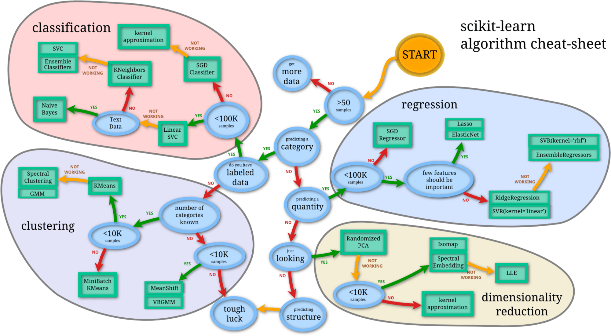
Choosing the right estimator in Scikit-Learn — Figure 1 – How to choose the right estimator in Scikit-Learn

Let us review the limitations that need to be considered when using several, well-known machine learning algorithms, starting with linear regression, and then progressing to other well-known algorithms such as logistic regression, decision trees, random forests, support vector machines, and gradient boosting.

Linear Regression #

Linear regression is a fundamental and widely used algorithm for predicting numerical values in machine learning. However, it has certain assumptions and limitations that need to be considered when using it. Here are some key issues to take into account when using linear regression:

Linearity Assumption: Linear regression assumes a linear relationship between the features and the target variable. If the relationship is non-linear, the model may not accurately capture the underlying patterns in the data. One useful tool for identifying non-linearity is the residual plot, where the residual is the differences between the actual and predicted values. If there is non-linearity in the data, then a simple correction may be to transform the predictor using log \(X\), \(\sqrt{X}\) or \(X^2\).
Homoscedasticity: Linear regression assumes that the variance of the errors (residuals) is constant across all levels of the predictor variables. If the data violates this assumption and exhibits heteroscedasticity, the model’s predictions may be less reliable for certain ranges of the input variables. One possible solution is to transform the outcome \(Y\) using a concave function such as log \(Y\) or \(\sqrt{Y}\).
Multicollinearity: Linear regression assumes that the predictor variables are not highly correlated with each other. If there is strong multicollinearity, it can reduce the accuracy of the regression coefficients, making it challenging to interpret the importance of individual features. The variance inflation factor can be employed to assess multicollinearity.
Outliers and high-leverage points: Linear regression is sensitive to outliers and high-leverage points, and a few of these extreme data points can have a significant impact on the model’s coefficients and predictions. The leverage statistics can attest if an observation is a high-leverage point.
Normality of Residuals: Linear regression assumes that the residuals are normally distributed. Departure from this assumption may affect the accuracy of statistical tests and confidence intervals.
Feature Scaling: When features have different scales, the linear regression algorithm can be influenced by the magnitude of the features. It is essential to scale the features appropriately to avoid any bias towards certain variables.
Overfitting and Underfitting: Linear regression can suffer from overfitting when the model is too complex relative to the amount of data available, or underfitting when it is too simple to capture the underlying patterns in the data. A possible path for understanding if the model is overfitting or underfitting is to plot a learning curve.
Presence of Non-Independence: Linear regression assumes that the observations are independent of each other. If the data exhibits autocorrelation or serial correlation (e.g., time series data), standard linear regression may not be appropriate.
Feature Engineering: Linear regression relies on feature engineering to capture non-linear relationships. If important non-linear patterns exist, you might need to add polynomial features or consider using other non-linear regression models.
Extrapolation: Linear regression is not suitable for extrapolation beyond the range of the observed data, as it assumes that the relationship between the features and the target variable holds within the observed range only.
Interpretability: Linear regression is relatively interpretable, as it provides straightforward coefficient estimates for each feature. However, for more complex problems with interactions between features, the interpretability might be limited.

To address some of these issues, one can explore alternative modeling approaches like non-linear regression, regularization techniques (e.g., Lasso, Ridge regression), or ensemble methods (e.g., Random Forest, Gradient Boosting) depending on the specific characteristics of the data and the complexity of the relationships between the features and the target variable.

Logistic Regression #

Logistic regression is a popular and widely used algorithm for binary classification tasks. However, like any machine learning method, it has its limitations and potential issues. Here are some key issues to consider when using logistic regression:

Linear Separability Assumption: Logistic regression assumes that the data are linearly separable, which means it can draw a straight line to separate the two classes. If the classes are not linearly separable, the model may not perform well.
Feature Independence: Logistic regression assumes that the features are independent of each other. If there are strong correlations between features, it might lead to multicollinearity, affecting the model’s stability and interpretability.
Outliers: Logistic regression can be sensitive to outliers, as they can disproportionately influence the model’s coefficients and decision boundary.
Imbalanced Data: When dealing with imbalanced datasets (i.e., one class is significantly more prevalent than the other), logistic regression may be biased towards the majority class, resulting in poor performance on the minority class. Techniques like resampling or using class weights can help mitigate this issue. Tools such as those described in the imbalanced-learn documentation can be of help.
Non-Linear Relationships: Logistic regression assumes a linear relationship between the features and the log-odds of the target variable. If the relationship is non-linear, the model might not capture complex patterns well.
Overfitting: If the number of features is large relative to the number of training samples, logistic regression may overfit the data, leading to poor generalization to new data.
Model Interpretability: While logistic regression is relatively interpretable, it may not capture complex interactions between features as effectively as more complex models.
Decision Threshold: The output of logistic regression is a probability value between 0 and 1. You need to choose a decision threshold to convert probabilities into class labels. The choice of the threshold affects the model’s precision and recall trade-off. To this end, the receiver operating characteristic curve, or ROC curve and the area under the curve (AUC) metrics may be of great help, as they can determine the threshold that produces the lowest false positive rate against the highest true positive rate.
Curse of Dimensionality: Logistic regression can suffer from the curse of dimensionality when the feature space becomes too high-dimensional, causing sparsity in the data.
Large Sample Size Requirements: In some cases, logistic regression may require a reasonably large sample size to generalize well and provide reliable estimates.
Feature Scaling: Logistic regression can be sensitive to feature scaling, so it’s important to scale the features appropriately to ensure convergence and stable model training.
Convergence Issues: During optimization, logistic regression may encounter convergence problems, especially when the features are highly correlated or when the learning rate is not well-tuned.

To address some of these issues, one can explore alternative modeling approaches, such as non-linear classifiers, ensemble methods, or deep learning models, depending on the complexity and characteristics of the data. Additionally, data preprocessing, feature engineering, and regularization techniques can help enhance the performance and stability of logistic regression.

Decision Trees #

When using decision trees, whether for regression or classification, there are several issues and considerations to keep in mind to ensure the model’s effectiveness and avoid potential pitfalls. Some of the key issues are as follows:

Overfitting: Decision trees are prone to overfitting, especially when they grow too deep and capture noise in the training data. Overfitting can lead to poor generalization on unseen data.
Tree Depth and Complexity: The depth of the decision tree impacts its complexity. Deep trees can become overly specific to the training data and might not generalize well, while shallow trees may not capture complex relationships.
Feature Importance: Decision trees may prioritize certain features over others, making them more critical in the decision-making process. It’s essential to assess feature importance to ensure the model is making decisions based on the most relevant features.
Sensitive to Small Variations: Decision trees can be sensitive to small changes in the data, which may result in different tree structures or predictions.
Imbalanced Data: Decision trees can be biased towards the majority class in imbalanced datasets, leading to poor performance on minority classes. Techniques like class weights or balancing the dataset can help address this issue. Once again, the tools in the imbalanced-learn documentation can be of help.
Handling Numerical Features: Traditional decision tree algorithms might not directly handle numerical features well. Techniques like discretization or using tree variants like CART (Classification and Regression Trees, which is the default in Scikit-Learn) can be used to handle numerical attributes.
Extrapolation: Decision trees are not suitable for extrapolation beyond the range of the training data, as they only make decisions based on the observed data.
Model Interpretability: Decision trees are inherently interpretable, but complex trees can be difficult to interpret. Using simpler trees or ensemble methods like Random Forest can improve interpretability.
Decision Boundary: Decision trees create piecewise-linear decision boundaries, which might not be optimal for some datasets with non-linear separability.
Ensemble Methods: While decision trees can be effective, using ensemble methods like Random Forest or Gradient Boosting can improve predictive performance and reduce overfitting.
Instability and Variance: Decision trees can exhibit instability, where small changes in the data can lead to significant changes in the tree’s structure and predictions.
Data Preprocessing: Decision trees are sensitive to the scale of features and outliers. Preprocessing techniques like feature scaling and outlier handling can affect the performance of the model.
Memory and Computational Complexity: Decision trees can grow large and consume significant memory, especially with deep trees or large datasets.
Missing Data Handling: Traditional decision tree algorithms might not handle missing data directly. Imputation techniques or tree variants that handle missing values can be used.

Addressing these issues may involve using techniques like pruning, setting maximum tree depth, using ensemble methods, or employing regularization to prevent overfitting and improve generalization. It is crucial to experiment with different hyperparameters and tree configurations to find the most suitable model for your specific problem.

Random Forests #

Random Forest is an ensemble learning method that combines multiple decision trees to improve predictive performance and reduce overfitting. They can be used both for classification and regression. While Random Forests are robust and widely used, there are still some issues and considerations to keep in mind when using them:

Overfitting: Although Random Forests are designed to reduce overfitting compared to individual decision trees, they can still overfit if the number of trees is excessively high or the trees are too deep.
Number of Trees: The number of trees in the forest is a hyperparameter that needs to be tuned. Too few trees may lead to underfitting, while too many trees can increase computation time and memory consumption.
Tree Depth and Complexity: Individual decision trees within the forest may still overfit the data if they are allowed to grow too deep. Limiting the tree depth or using techniques like tree pruning can help control complexity.
Feature Importance Interpretation: While Random Forests provide a measure of feature importance, interpreting the significance of feature importance values for highly correlated features can be challenging.
Computational Resources: Random Forests can be computationally expensive, especially with a large number of trees or deep trees. Training and predicting with large ensembles may require significant computational resources.
Handling Numerical Features: Random Forests can handle numerical features naturally, but they may not work well with categorical features with high cardinality. One-hot encoding or other encoding techniques might be required.
Imbalanced Data: Random Forests can still be biased towards the majority class in imbalanced datasets. Techniques like class weights, data balancing, or adjusting decision thresholds can be applied to address this issue.
Out-of-Bag (OOB) Samples: Random Forests use out-of-bag samples to estimate model performance during training. However, OOB estimates might not be as accurate as cross-validation, especially for small datasets.
Memory Consumption: Ensembles with a large number of trees can consume substantial memory, limiting their usability in memory-constrained environments.
Extrapolation: Random Forests, like decision trees, are not suitable for extrapolation beyond the range of the training data.
Ensemble Size vs. Performance: In some cases, increasing the number of trees beyond a certain point might not significantly improve performance but will increase training time and memory usage.
Dependency on Data Size and Quality: Random Forests may not perform well on small or poor-quality datasets, as they rely on the diversity of trees for better performance.
Training Time: Training a Random Forest can take longer compared to individual decision trees, especially when the dataset is large.

To address these issues, it’s essential to properly tune the hyperparameters, limit tree depth, monitor and control overfitting, handle imbalanced data, and select an appropriate number of trees. Additionally, using feature selection techniques or exploring other ensemble methods (e.g., Gradient Boosting) might be beneficial in certain scenarios.

Support Vector Machines #

Support Vector Machines (SVMs) are powerful and versatile machine learning algorithms for both classification and regression tasks. However, they come with their own set of issues and considerations. Here are some key issues to take into account when using Support Vector Machines:

Kernel Selection and Parameters: SVMs often require the use of kernel functions to handle non-linearly separable data. Selecting the appropriate kernel and tuning its parameters can significantly impact the model’s performance.
Data Scaling: SVMs are sensitive to the scale of the features. It’s crucial to scale the data properly to avoid certain features dominating the optimization process.
Computational Complexity: Training SVMs can be computationally expensive, especially for large datasets. The time and memory requirements increase with the number of data points and features.
Memory Consumption: The memory requirements for SVMs can be substantial, especially when using non-linear kernels or large datasets.
Sensitivity to Outliers: SVMs are sensitive to outliers at the margins as they can affect the placement of the decision boundary.
Interpretability: SVMs can be less interpretable than linear models due to the complexity of the decision boundary, especially when using non-linear kernels.
Choice of Regularization Parameter (C): The regularization parameter (C) controls the trade-off between maximizing the margin and minimizing the classification error. The optimal value of C depends on the data and problem at hand.
Class Imbalance: SVMs can be biased towards the majority class in imbalanced datasets, leading to suboptimal performance for the minority class. Techniques like class weights or using different kernels can help address this issue.
Large Number of Features: SVMs may not perform well with high-dimensional data, as the computational complexity increases with the number of features.
Memory and Time Complexity during Prediction: Predicting with SVMs can also be computationally expensive, especially with large-scale problems.
Handling Large Datasets: Training SVMs on large datasets might be impractical due to the computational and memory requirements. In such cases, approximate methods or kernel approximation techniques can be used.
Noise Sensitivity: SVMs can be sensitive to noisy data, which might lead to overfitting.
Cross-Validation and Parameter Selection: Proper cross-validation and parameter tuning are critical for achieving optimal SVM performance.
Binary Classification Limitation: SVMs are inherently binary classifiers. To use SVMs for multi-class problems, techniques like One-vs-One or One-vs-Rest are applied.
Data Preprocessing: Appropriate data preprocessing, including handling missing values and outliers, is crucial for SVM performance.

To mitigate some of these issues, practitioners often perform feature selection, use efficient libraries and optimization algorithms, perform cross-validation, and preprocess data to handle outliers and missing values effectively. Additionally, selecting the right kernel and tuning hyperparameters are essential for achieving better SVM performance. If the data is too large or computationally intensive, alternative methods like stochastic gradient descent or kernel approximation techniques may be considered.

Gradient Boosting #

Gradient Boosting is a powerful ensemble learning technique that combines multiple weak learners (typically decision trees) to create a strong predictive model. While gradient boosting algorithms like XGBoost and LightGBM have shown remarkable performance across various tasks, there are certain issues and considerations to be aware of when using them:

Overfitting: Gradient boosting models are prone to overfitting, especially when the number of trees (boosting iterations) is too high or the trees are too deep. Regularization techniques like learning rate and tree depth limitations can help mitigate overfitting.
Computational Complexity: Gradient boosting can be computationally expensive, especially with a large number of trees and high-dimensional feature spaces.
Memory Consumption: Gradient boosting models can consume significant memory, especially when the datasets are large or when using large tree ensembles.
Hyperparameter Tuning: Proper hyperparameter tuning is crucial for achieving the best model performance. However, the tuning process can be time-consuming and computationally expensive.
Data Scaling: Gradient boosting models are generally not sensitive to feature scaling. However, scaling might affect the optimization process for specific hyperparameters.
Outliers: Gradient boosting models can be sensitive to outliers, especially when using shallow trees. Preprocessing techniques to handle outliers can be beneficial.
Gradient Exploding/Vanishing: During the training process, gradients might explode (become too large) or vanish (become too small), affecting the model’s convergence. Careful regularization and proper learning rate can help address this issue.
Imbalanced Data: Gradient boosting can be biased towards the majority class in imbalanced datasets, leading to suboptimal performance on minority classes. Techniques like class weights or balanced sampling can be employed to handle imbalanced data.
Feature Importance Interpretation: While gradient boosting models provide feature importance scores, interpreting them for highly correlated features can be challenging.
Interpretability: Gradient boosting models are less interpretable compared to linear models or decision trees, especially with deep ensembles.
Non-linear Relationships: Gradient boosting models can capture non-linear relationships between features and the target variable. However, if the relationships are highly complex, a large number of trees might be required, leading to increased training time and memory usage.
Extrapolation: Like decision trees, gradient boosting models are not suitable for extrapolation beyond the range of the training data.
Data Preprocessing: Proper data preprocessing, including handling missing values and encoding categorical variables, is essential for optimal model performance.
Ensemble Size vs. Performance: In some cases, increasing the number of boosting iterations beyond a certain point might not significantly improve performance but will increase training time and memory usage.

Addressing these issues involves a combination of hyperparameter tuning, regularization techniques, handling imbalanced data, appropriate data preprocessing, and monitoring model complexity to prevent overfitting. Despite these challenges, gradient boosting remains one of the most effective and popular machine learning techniques for a wide range of tasks.